We present a comparison between autoencoders and variational autoencoders. For this, we describe their
architecture and explain the respective advantages. To gain a deeper insight into the encoding and decoding
process, we visualize the distribution of values in latent space for both models. While autoencoders are
commonly used for compression, variational autoencoders typically act as generative models. We provide an
interactive visualization to explore their differences. By manually modifying the latent activations, the user
can directly observe the impact of different latent values on the generated output.
In addition, we provide an information theoretic view on the compressive properties of autoencoders.
Introduction
For the past few years, autoencoding and generative models have played an important role in unsupervised machine
learning and deep learning in particular. Introduced by , an autoencoder is a
special type of a neural network with two main characteristics:
The network is trained to output its own inputs.
The hidden layers of the network are significantly smaller than input and output layers.
Figure 1 shows the schematical layout of an autoencoder (AE). It consists of two parts,
the encoder and the decoder. The encoder decreases the dimensionality of the input up to the layer
with the fewest neurons, called latent space. The decoder then tries to reconstruct the input from this
low-dimensional representation. This way, the latent space forms a bottleneck, which forces the autoencoder to
learn an effective compression of the data.
Figure 1:
Network topology of an autoencoder. The hidden layers are smaller than input and output layers. The hidden
layer with the fewest neurons is called latent space. Since the network is trained to output its
input, latent space is the point where the network is supposed to find the best possible compression of the
data.
The capability to compress data can be used for a variety of tasks and different types of data: train an AE to remove noise from images, whereas
present a lossy image compression algorithm based
on AEs. use an AE for machine translation.
Variational Autoencoder
Despite the many applications of AEs, there is no way to predict the distribution of values in latent space.
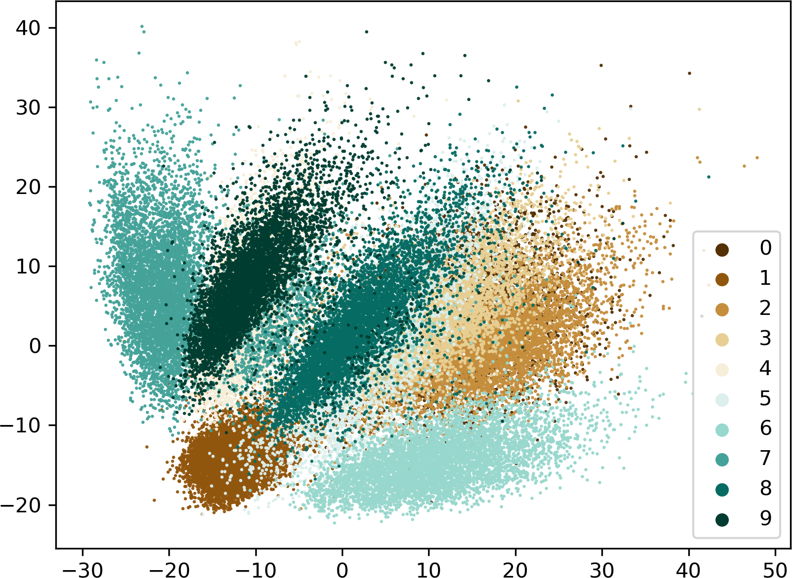
Typically, the latent space is sparsely populated, as shown in Figure 4a. This does
not impose a problem for compression systems, since it does not limit the compression factor that can be
reached. In contrary, scattered values indicate an ideal utilization of the available space and often lead to
better reconstruction results at high compression ratios. However, for generating new images this sparsity is an
issue, since finding a latent value for which the decoder knows how to produce valid output is unlikely.
To overcome these limitations, we need a way to gain more control over the latent space, making it more
predictable. This is where variational autoencoders (VAE) come into play. Since we are dealing with neural
networks, which are trained using gradient descent algorithms, the most straightforward approach is to introduce
an additional optimization target that aims to limit the chaos in latent space.
VAEs achieve this by forcing the latent variables to become normally distributed. Instead of passing the output
of the encoder directly to the decoder, we use it to form the parameters mean \(\mu \) and standard deviation
\(\sigma \) of a normal distribution \(\mathcal{N}(\mu,\sigma^2)\). The latent activations are then generated by
sampling from this distribution. Figure 2 shows the architecture of a VAE.
Using the encoder output as \(\mu \) and \(\sigma \) is not sufficient to make our latent space well-behaved.
the network would simply adjust \(\mu \) to the latent activations of the standard AE. To avoid this, we define
the standard normal distribution \( \mathcal{N}(0,1) \) as target reference during optimization. The distance
between our learned distribution and the standard normal distribution can be quantified using the
Kullback–Leibler (KL) divergence. It measures how much one probability distribution diverges from a second . During training, we force our normal
distribution as close as possible to the standard normal distribution by including the KL divergence in our loss
function.
Figure 2:
The variational autoencoder tries to limit the chaos in AEs latent-space by forcing the latent activations
to be normally distributed. This is done by using the encoder output as parameters \(\mu \) and \(\sigma \)
of a normal distribution. The latent activation then is generated by sampling from this distribution. During
training, the distribution is optimized to resemble a standard normal distribution as good as possible while
still producing reasonable reconstruction results.
The loss function now consists of two terms: The KL-loss and the reconstruction loss. Calculating the gradient
with regard to the KL-loss is straight forward, since it is analytically computable and only depends on the
parameters of the distributions.
For the reconstruction loss, things are different. The reconstruction is based on a random sample, which raises
the question: Does drawing random samples have a gradient? Obviously, the answer to this question is no, since
drawing samples is a random process with single, discrete outcomes.
To solve this issue, , the authors of the
original paper on the variational autoencoder, propose a method called reparameterization trick. Instead
of directly drawing random samples from a normal distribution $\mathcal{N}(\mu, \sigma^2)$, they make use of the
fact that every normal distribution can be expressed in terms of the standard normal distribution
$\mathcal{N}(0, 1)$: \[ \mathcal{N}(\mu, \sigma^2) \sim \mu + \sigma^2 \cdot \mathcal{N}(0, 1) \] When
processing an input image, we can make use of this property by drawing a sample $\epsilon$ from the standard
normal distribution and transform it to a latent sample $z$: \[z = \mu + \sigma^{2} \cdot \epsilon, \quad
\epsilon \leftarrow \mathcal{N}(0, 1)\] At first, this rewrite does not seem to help much with our problem. But
if we take a closer look, it separates the random component from the parameters that we are trying to learn, as
shown in Figure 3.
(a)
Before applying reparameterization trick
(b)
After applying reparameterization trick
Figure 3:
The sampling process in latent space before (a), and after applying the reparameterization trick (b). In
(a), the random, discrete outcome of $z$ prevents backpropagation over the parameters of the normal
distribution $\mu$ and $\sigma$. The reparameterization in (b) allows calculating a gradient over $\mu$ and
$\sigma$, since the last remaining random component is $\epsilon$, which can be treated as a constant per
sample.
Since we have factored out the randomness, we can now compute gradients with respect to $\mu$ and $\sigma$!
Ultimately, to update our weights, we have to get rid of the remaining random component $\epsilon$. This is done
by utilizing the law of large numbers :
even if we treat $\epsilon$ as a constant for each training sample, since our training data set is huge, we
expect the introduced error to average out over all samples. This procedure of solving complex problems
numerically by performing a large number of stochastic experiments is called Monte Carlo method .
If you are interested in the details of the algorithm introduced by , feel free
to have a look at the more advanced explanation by .
Extensions to VAEs
Despite VAEs allowing easy generation of meaningful new outputs, the results often suffer from a lack of detail.
provide a solution to this problem by using a different
distance function then the Kullback-Leibler divergence. The dense compression of data in latent space also
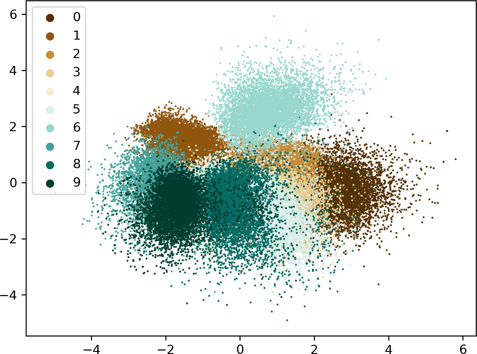
allows clustering models based on VAEs as shown by . To get an intuition why
this might work quite well have a closer look at Figure 4b.
Visualizing Latent-Space
We believe that visualization is a good way to show the characteristics of VAEs and helps to understand the
differences to traditional AEs. Therefore we trained an AE and the corresponding VAE on the MNIST dataset. The
dataset consists of 60,000 images of handwritten digits. Both AE and VAE share the same architecture with a
four-dimensional latent space. While designing our networks, we chose a tradeoff between visual explicability
and reconstruction accuracy.
To get an initial understanding of the distribution in latent space, we reduce the latent vectors of all
training images to two dimensions using a principal component analysis (PCA). The results are visualized using
scatter plots in Figure 4.
(a)
Latent Distribution by Label for AE
(b)
Latent Distribution by Label for VAE
Figure 4:
The distribution of latent values over the whole training data set both for AE (a) and VAE (b). In order to
visualize the four-dimensional latent activations, a principal component analysis was applied to transform
them into 2D space. Each color represents a different digit from the dataset. The diagram gives insight into
the spatial distribution of the latent values. While the AE builds up large, mutually independent clusters
over large ranges, the VAEs values are (by design) distributed around the origin. They build up smaller,
spherical clusters which are contiguous and share a similar value range. This shows the advantages of VAEs
in terms of generating new content: the room, which has to be filled with random values is much more compact
compared to the AEs.
To gain further insights we visualize the four latent variables in a parallel coordinate system, in which we
allow the user a direct manipulation of the activations. The latent activations are directly derived from the
input images on the left, which are passed to the encoder. If more than one input image is selected, the latent
activation is plotted for each image individually, marked by different colors.
The black line is the reconstruction line. Its values are taken as input for the decoder, whose image output is
rendered on the right. By manually dragging the points of the reconstruction line, the latent variables passed
to the decoder can be altered. Double-clicking an input activation line snaps the output activation to this
line.
In the default state, only the activations of the VAE are displayed. By clicking the checkbox "Show AE", the VAE
values get greyed out and the latent activations of the AE will be shown. The grey violin plots in the
background depict the underlying frequency distribution over the whole training dataset. By clicking the dice
icon labeled Random, the output activation is set by drawing random samples from a normal distribution,
clipped to the visible space.
Please note that the MNIST-images are inverted (black on white) in this figure to improve readability. The
network was trained on the original white-on-black images of the MNIST dataset. The questionmark , the letter and the stickman are not part of the dataset. They
are provided to allow testing images that are totally new to the network.
Interesting Findings
Our visualization illustrates the large difference between AEs and VAEs regarding their behavior in latent
space. For the given input images, the value range in latent space is \([-5.93, 5.98]\) for the VAE in
contrast to \([-22.59, 74.46]\) for the AE.
This makes clear why generating new content with AEs is difficult. To come up with new latent vectors, we
need a lot of luck to find a value for which the decoder knows a useful reconstruction. In case of our VAE,
we simply need to draw random samples from a standard normal distribution with a good chance that the
decoder produces valid output.
With respect to the full range in which latent values occur, the VAE produces reasonable outputs over a
larger range than the AE.
To our own surprise, interpolations between multiple images work quite well with both VAE and AE.
It is interesting where the compression locates values in latent space. By just modifying the value of a
single dimension, it is possible to generate multiple images of different digits.
Drawbacks and Limitations of VAEs
The advantages of VAEs come at a cost. Since we penalize the network for learning latent representations which
are very unlikely to be drawn from a standard normal distribution, we limit the amount of information that can
be stored in latent space. Therefore, compared to a VAE, a standard AE reaches a far better compression ratio.
It is already difficult to produce acceptable reconstructions with the four latent variables of the above VAE,
while we have achieved equally good results with an AE reduced to only two latent variables.
An Information Theoretic View
Regarding information theory, this behavior is not surprising. Our input images have a size of $32 \times 32$
pixels with one color channel (grayscale). Each pixel can take integer values from $[0, 255]$. Therefore one
input image stores \[32 \cdot 32 \cdot 1 \cdot \log_2(256) = 8192 \textrm{ bits} \] of information. Considering
the precision of $32 \textrm{ bit}$ floating point values, our network architecture can encode \(32 \textrm{
bit} \cdot 4 = 128 \textrm{ bits} \) in its four latent variables. This is only a factor of \(8192 \textrm{
bits} / 128 \textrm{ bits} = 64 \) less than our input images.
In other words, with an ideal encoding in latent space, we could perfectly reconstruct arbitrary images with a
chance of \(1/64 \approx 1.56\% \). At first, this does not seem to be a very good reconstruction rate but we
have to consider that:
we are talking about a perfect reconstruction, i.e. every pixel in the output image is exactly the same as
in the input image.
the images in our dataset (MNIST) have great similarities. Some pixels (corners and borders) are actually
always black.
This explains why the AE performs well at compressing our data. For the VAE, the additional constraint limits
the information density that can be reached in latent space by making a broad range of the $32 \textrm{ bit}$
floating point values very unlikely to occur.
Please note that a network will never reach a perfect encoding as the one mentioned above. The performance of a
real network is heavily limited by architecture, weight initialization, and optimization algorithm. The above
calculation is only used to give an intuition for the amount of information that is encoded in the different
stages of an AE/VAE.
Conclusion
Our visualization gives access to an otherwise covert part of autoencoders and variational autoencoders by
enabling interaction with the latent space. By visualizing the core of their mechanism we can gain insight into
the way their compression works.
Neural networks are probably one of the most powerful and promising approaches in the field of machine learning.
Despite the restrictions mentioned in the previous chapter, they can be applied to data from a variety of
domains and are able to adapt to many different tasks. The compression reached by AEs is remarkable: if our
network can reconstruct MNIST samples from only four latent activations, this equates to a compression ratio of
$≈ 98.5 \%$. The network reminds the essence of the dataset. And, in the case of generative algorithms such as
our VAE, it can even come up with new results.
Further reading
If you are interested in writing your own AE/VAE, consider having a look at the blog posts by and .
References
Acknowledgements
We would like to thank the German Research Foundation (DFG) for financial support within project A01 of the SFB-TRR
161.


 , the letter
  and the stickman
  are not part of the dataset. They
are provided to allow testing images that are totally new to the network.
are not part of the dataset. They
are provided to allow testing images that are totally new to the network.